Step-by-Step Solutions to Common Examples of Linear Transformations in Linear Algebra

Linear transformations allow us to use matrices to describe how vectors move, stretch, rotate, and reflect through space. In this article, we’ll explore examples of linear transformations in linear algebra, showing how each works and how to represent them using matrices. By the end, you’ll understand what a transformation is and how to apply it to vectors in $ \mathbb{R}^2 $ and $ \mathbb{R}^3 $.

In this guide, we’ll start by defining what makes a transformation linear and then walk through the most common types of transformations, including reflections, projections, dilations, and rotations, in two and three dimensions. Using matrix multiplication, you’ll also learn how to compose or apply several transformations in sequence.

This guide uses concepts covered in the articles The Ultimate Step-by-Step Guide to Basic Matrix Operations for Beginners and Vector Operations Tutorial for Beginners: A Complete Step-by-Step Guide, so please read them if you haven’t already.

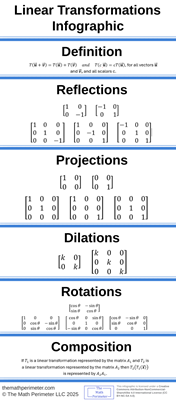
The following infographic illustrates the concepts covered in this article.

Linear Transformations Infographic Resized. Related Article - Step-by-Step Solutions to Common Examples of Linear Transformations in Linear Algebra.

View Full Size Infographic

What Is a Linear Transformation?

A transformation $ T: \mathbb{R}^n \to \mathbb{R}^m $ is linear if, for any vectors $ \mathbf{u}, \mathbf{v} \in \mathbb{R}^n $ and any scalar $ c \in \mathbb{R} $, the following two properties hold:

$$T(\mathbf{u} + \mathbf{v}) = T(\mathbf{u}) + T(\mathbf{v})$$

$$T(c\mathbf{u}) = cT(\mathbf{u}).$$

Matrix Representation of a Linear Transformation

Every linear transformation can be represented by a matrix. If $ T $ is a linear transformation from $ \mathbb{R}^n $ to $ \mathbb{R}^m $, then there exists an $ m \times n $ matrix $ A $ such that for every vector $ \mathbf{x} \in \mathbb{R}^n $:

$$T(\mathbf{x}) = A\mathbf{x}$$

Here, $ A $ is called the induced matrix of the linear transformation. Each column of $ A $ represents how $ T $ acts on one of the basis vectors of $ \mathbb{R}^n $.

Common Linear Transformations in $ \mathbb{R}^2 $

Linear transformations in $ \mathbb{R}^2 $ can be described using $ 2 \times 2 $ matrices. These matrices determine how vectors are transformed. Each transformation alters the vector in some way, but preserves linearity.

Below, we’ll go through the most common transformations in $ \mathbb{R}^2 $.

Reflections in $ \mathbb{R}^2 $

Reflection across the $ x $-axis

$$\begin{bmatrix}
1 & 0 \\
0 & -1
\end{bmatrix}.$$

Reflection across the $ y $-axis

$$\begin{bmatrix}
-1 & 0 \\
0 & 1
\end{bmatrix}.$$

Projections in $ \mathbb{R}^2 $

Projection onto the $ x $-axis

$$\begin{bmatrix}
1 & 0 \\
0 & 0
\end{bmatrix}.$$

Projection onto the $ y $-axis

$$\begin{bmatrix}
0 & 0 \\
0 & 1
\end{bmatrix}.$$

Dilation in $ \mathbb{R}^2 $

$$\begin{bmatrix}
k & 0 \\
0 & k
\end{bmatrix}.$$

Rotation in $ \mathbb{R}^2 $

$$\begin{bmatrix}
\cos \theta & -\sin \theta \\
\sin \theta & \cos \theta
\end{bmatrix}.$$

Common Linear Transformations in $ \mathbb{R}^3 $

Linear transformations in $ \mathbb{R}^3 $ extend the same principles we saw in $ \mathbb{R}^2 $, but now vectors can rotate or reflect through three-dimensional space. Each transformation is represented by a $ 3 \times 3 $ matrix, which determines how points change along the $ x $-, $ y $-, and $ z $-axes.

We’ll now look at the most common types of linear transformations in $ \mathbb{R}^3 $.

Reflections in $ \mathbb{R}^3 $

Reflection across the $ xy $-plane

$$\begin{bmatrix}
1 & 0 & 0 \\
0 & 1 & 0 \\
0 & 0 & -1
\end{bmatrix}.$$

Reflection across the $ yz $-plane

$$\begin{bmatrix}
-1 & 0 & 0 \\
0 & 1 & 0 \\
0 & 0 & 1
\end{bmatrix}.$$

Reflection across the $ xz $-plane

$$\begin{bmatrix}
1 & 0 & 0 \\
0 & -1 & 0 \\
0 & 0 & 1
\end{bmatrix}.$$

Projections in $ \mathbb{R}^3 $

Projection onto the $ xy $-plane

$$\begin{bmatrix}
1 & 0 & 0 \\
0 & 1 & 0 \\
0 & 0 & 0
\end{bmatrix}.$$

Projection onto the $ xz $-plane

$$\begin{bmatrix}
1 & 0 & 0 \\
0 & 0 & 0 \\
0 & 0 & 1
\end{bmatrix}.$$

Projection onto the $ yz $-plane

$$\begin{bmatrix}
0 & 0 & 0 \\
0 & 1 & 0 \\
0 & 0 & 1
\end{bmatrix}.$$

Dilation in $ \mathbb{R}^3 $

$$\begin{bmatrix}
k & 0 & 0 \\
0 & k & 0 \\
0 & 0 & k
\end{bmatrix}.$$

Rotations in $ \mathbb{R}^3 $

Rotation about the $ x $-axis

$$\begin{bmatrix}
1 & 0 & 0 \\
0 & \cos \theta & -\sin \theta \\
0 & \sin \theta & \cos \theta
\end{bmatrix}.$$

Rotation about the $ y $-axis

$$\begin{bmatrix}
\cos \theta & 0 & \sin \theta \\
0 & 1 & 0 \\
-\sin \theta & 0 & \cos \theta
\end{bmatrix}.$$

Rotation about the $ z $-axis

$$\begin{bmatrix}
\cos \theta & -\sin \theta & 0 \\
\sin \theta & \cos \theta & 0 \\
0 & 0 & 1
\end{bmatrix}.$$

Composition of Linear Transformations

If $ T_1 $ and $ T_2 $ are linear transformations from $ \mathbb{R}^n $ to $ \mathbb{R}^n $, and if $ A_1 $ and $ A_2 $ are their respective matrices, then applying $ T_1 $ followed by $ T_2 $ is written as

$$T(\mathbf{x}) = T_2(T_1(\mathbf{x})).$$

The matrix for the composite transformation $ T $ is given by

$$A = A_2 A_1.$$

Notice that the order of multiplication matters. Because matrix multiplication is not commutative, the order in which transformations are applied affects the result.

Worked Out Example

Example 1: (a) Transform the vector $ \langle 1, 0 \rangle $ by first rotating by $ 90^\circ $, them dilating by a factor of 2.
(b) Transform the vector $ \langle 1, 0, 1 \rangle $ by reflecting across the xy-plane, then rotating by $ 90^\circ $ about the z-axis.

Solution: (a) Transform the vector $ \langle 1, 0 \rangle $ by first rotating by $ 90^\circ $, them dilating by a factor of 2.

The rotation matrix is

$$\begin{bmatrix}
0 & -1 \\
1 & 0
\end{bmatrix},$$

and the dilation matrix is

$$\begin{bmatrix}
2 & 0 \\
0 & 2
\end{bmatrix}.$$

Hence, we need to compute

$$\begin{bmatrix}
2 & 0 \\
0 & 2
\end{bmatrix}
\begin{bmatrix}
0 & -1 \\
1 & 0
\end{bmatrix}
\begin{bmatrix}
1 \\
0
\end{bmatrix}.$$

Performing matrix multiplication, we get

$$\begin{bmatrix}
2(0) + 0(1) & 2(-1) + 0(0) \\
0(0) + 2(1) & 0(-1) + 2(0)
\end{bmatrix}
\begin{bmatrix}
1 \\
0
\end{bmatrix}.$$

Multiplying we obtain

$$\begin{bmatrix}
0 + 0 & -2 + 0 \\
0 + 2 & 0 + 0
\end{bmatrix}
\begin{bmatrix}
1 \\
0
\end{bmatrix}.$$

Adding we have

$$\begin{bmatrix}
0 & -2 \\
2 & 0
\end{bmatrix}
\begin{bmatrix}
1 \\
0
\end{bmatrix}.$$

Performing matrix multiplication again, we get

$$\begin{bmatrix}
0(1) – 2(0) \\
2(1) + 0(0)
\end{bmatrix}.$$

Multiplying we obtain

$$\begin{bmatrix}
0 – 0 \\
2 + 0
\end{bmatrix}.$$

Adding and subtracting, we arrive at

$$\begin{bmatrix}
0 \\
2
\end{bmatrix}.$$

The final transformed vector is then

$$\langle 0, 2 \rangle.$$

(b) Transform the vector $ \langle 1, 0, 1 \rangle $ by reflecting across the xy-plane, then rotating by $ 90^\circ $ about the z-axis.

The reflection matrix is

$$\begin{bmatrix}
1 & 0 & 0 \\
0 & 1 & 0 \\
0 & 0 & -1
\end{bmatrix},$$

and the rotation matrix is

$$\begin{bmatrix}
0 & -1 & 0 \\
1 & 0 & 0 \\
0 & 0 & 1
\end{bmatrix}.$$

Hence, we need to compute

$$\begin{bmatrix}
0 & -1 & 0 \\
1 & 0 & 0 \\
0 & 0 & 1
\end{bmatrix}
\begin{bmatrix}
1 & 0 & 0 \\
0 & 1 & 0 \\
0 & 0 & -1
\end{bmatrix}
\begin{bmatrix}
1 \\
0 \\
1
\end{bmatrix}.$$

Performing matrix multiplication, we get

$$\begin{bmatrix}
0(1) – 1(0) + 0(0) & 0(0) – 1(1) + 0(0) & 0(0) – 1(0) + 0(-1) \\
1(1) + 0(0) + 0(0) & 1(0) + 0(1) + 0(0) & 1(0) + 0(0) + 0(-1) \\
0(1) + 0(0) + 1(0) & 0(0) + 0(1) + 1(0) & 0(0) + 0(0) + 1(-1)
\end{bmatrix}
\begin{bmatrix}
1 \\
0 \\
1
\end{bmatrix}.$$

Multiplying we obtain

$$\begin{bmatrix}
0 – 0 + 0 & 0 – 1 + 0 & 0 – 0 + 0 \\
1 + 0 + 0 & 0 + 0 + 0 & 0 + 0 + 0 \\
0 + 0 + 0 & 0 + 0 + 0 & 0 + 0 – 1
\end{bmatrix}
\begin{bmatrix}
1 \\
0 \\
1
\end{bmatrix}.$$

Adding and subtracting, we have

$$\begin{bmatrix}
0 & -1 & 0 \\
1 & 0 & 0 \\
0 & 0 & -1
\end{bmatrix}
\begin{bmatrix}
1 \\
0 \\
1
\end{bmatrix}.$$

Performing matrix multiplication again, we get

$$\begin{bmatrix}
0(1) – 1(0) + 0(1) \\
1(1) + 0(0) + 0(1) \\
0(1) + 0(0) – 1(1)
\end{bmatrix}.$$

Multiplying we obtain

$$\begin{bmatrix}
0 – 0 + 0 \\
1 + 0 + 0 \\
0 + 0 – 1
\end{bmatrix}.$$

Adding and subtracting, we arrive at

$$\begin{bmatrix}
0 \\
1 \\
-1
\end{bmatrix}.$$

The final transformed vector is then.

$$\langle 0, 1, -1 \rangle.$$

Conclusion

In this guide, we explored some of the most common examples of linear transformations in linear algebra, including reflections, rotations, dilations, and projections in $ \mathbb{R}^2 $ and $ \mathbb{R}^3 $. Each transformation can be expressed using a matrix, allowing us to compute how vectors change under various transformations. By composing transformations, we can build more complicated transformations through matrix multiplication.

Frequently Asked Questions

No. Translations are not linear transformations because they do not preserve the origin.

Step-by-Step Solutions to Common Examples of Linear Transformations in Linear Algebra