Separable Differential Equations Explained Step by Step: A Complete Beginner’s Guide
One of the first techniques encountered in the study of differential equations is the method of separation of variables. In this guide, on separable differential equations explained step by step, you will learn how to recognize separable equations, understand why the method of separation of variables works, and apply it to solve separable differential equations.
In this article, we will begin by defining separable differential equations and explain how to identify them. Next, we will derive the general solution method directly from the differential equation and explain why separation of variables yields a valid solution. We will then present a step-by-step procedure that you can follow for any separable differential equation. Finally, we will work through several detailed examples. By the end of this guide, you will have a solid understanding of how to solve separable differential equations.
What Are Separable Differential Equations?
Before learning how to solve separable differential equations, it is important to understand what they are and how to recognize them.
Like any differential equation, separable differential equations contain derivatives. If you need a review of derivatives, please refer to the article How to Differentiate a Function Step by Step: A Beginner’s Guide before continuing.
Definition
A separable differential equation is a first-order differential equation that can be written in the form
$$\frac{dy}{dx}=f(x)g(y),$$
where \( f(x) \) is a function of \( x \) only and \( g(y) \) is a function of \( y \) only.
Implicit vs Explicit Solution
An implicit solution has the form \( y = f(x) \), whereas an explicit solution does not.
Derivation
In this section, we will derive the solution method directly from the general form of a separable differential equation. Understanding this derivation helps explain why the procedure of separating variables and integrating both sides produces valid solutions.
For a review of integration, please refer to the article Basic Integration Problems for Beginners.
Recall that a separable differential equation can be written as
$$\frac{dy}{dx}=f(x)g(y),$$
where \( f(x) \) depends only on \( x \) and \( g(y) \) depends only on \( y \).
Our goal is to determine the unknown function that satisfies this equation. To begin, we want to place all terms involving \( y \) on one side and all terms involving \( x \) on the other. Assuming \( g(y)\neq 0 \), divide both sides by \( g(y) \):
$$\frac{1}{g(y)}\frac{dy}{dx}=f(x).$$
Next, multiply both sides by \( dx \):
$$\frac{1}{g(y)}\,dy=f(x)\,dx.$$
This step separates the variables. The left side now contains only expressions involving \( y \), while the right side contains only expressions involving \( x \).
Once the variables have been separated, we integrate both sides:
$$\int \frac{1}{g(y)}\,dy = \int f(x)\,dx + C.$$
Because the variables have been isolated, each integral can be evaluated independently. In many cases, this equation is left in this form once the integrals are evaluated. Such a solution is called an implicit solution because \( y \) is not isolated. Sometimes it is possible to solve for \( y \) explicitly. Depending on the problem, the solution may remain implicit or be rewritten explicitly. If an initial condition is provided, it can be used to determine the value of the constant and obtain a particular solution.
Step-by-Step Procedure for Solving Separable Differential Equations
Now that we understand both the definition of a separable differential equation and the solution method, we can develop a systematic procedure for solving them. Although individual problems may vary in complexity, the overall strategy remains the same.
Step 1: Determine Whether the Equation Is Separable
Look for an equation that can be written in the form
$$\frac{dy}{dx}=f(x)g(y).$$
In some cases, the equation will already appear in this form. In other cases, algebraic manipulation may be required before the separable structure becomes obvious.
Step 2: Separate the Variables
Once the equation is in the proper form, move all terms involving \( y \) to one side and all terms involving \( x \) to the other.
Step 3: Integrate Both Sides
After isolating the variables, integrate each side with respect to its variable, and introduce a constant of integration on the right-hand side. At this stage, the differential equation has been solved in implicit form.
Step 4: Solve for \( y \) If Possible
Depending on the equation, it may be possible to isolate \( y \). When \( y \) can be isolated, the result is called an explicit solution.
Step 5: Apply the Initial Condition (If Given)
Substitute the given values into the general solution and solve for the constant of integration.
Worked Out Examples
The best way to learn the separation of variables method is through practice. In this section, we will work through five examples.
Example 1: Solve \( \frac{dy}{dx}=xy \).
Solution: The equation is already in standard form. Separating variables, we have
$$\frac{1}{y} dy = x dx.$$
Integrating both sides, we find
$$\int \frac{1}{y} dy = \int x dx.$$
Therefore
$$\ln|y| = \frac{1}{2}x^2 + C.$$
In exponential form, this is
$$|y| = e^{\frac{1}{2}x^2 + C}.$$
Using exponential properties, we obtain
$$|y| = e^{\frac{1}{2}x^2}e^C.$$
This is equivalent to
$$|y| = Ce^{\frac{1}{2}x^2}.$$
Dropping the absolute value bars then gives
$$y = \pm Ce^{\frac{1}{2}x^2}.$$
Our final solution is then
$$y = Ce^{\frac{1}{2}x^2}.$$
The next example requires the substitution rule, so you may wish to review the article The Ultimate Step-by-Step Guide to Solving Integrals Using Substitution for a refresher.
Example 2: Solve \( \frac{dy}{dx} = \frac{x(y^2 + 1)}{2y} \).
Solution: The equation is already in standard form. Separating variables, we have
$$\frac{2y}{y^2 + 1} dy = x dx.$$
Integrating both sides, we find
$$\int \frac{2y}{y^2 + 1} dy = \int x dx.$$
To evaluate the integral on the left-hand side, let \( u = y^2 + 1 \). Computing the differential gives \( du = 2y dy \). Substituting these into the integral, we arrive at
$$\int \frac{1}{u} du = \int x dx.$$
Integrating, we obtain
$$\ln|u| = \frac{1}{2}x^2 + C.$$
Therefore
$$\ln|y^2 + 1| = \frac{1}{2}x^2 + C.$$
In exponential form, this is
$$|y^2 + 1| = e^{\frac{1}{2}x^2 + C}.$$
Using exponential properties, we obtain
$$|y^2 + 1| = e^{\frac{1}{2}x^2}e^C.$$
This is equivalent to
$$|y^2 + 1| = Ce^{\frac{1}{2}x^2}.$$
Dropping the absolute value bars then gives
$$y^2 + 1 = Ce^{\frac{1}{2}x^2}.$$
Subtracting 1 from both sides, we get
$$y^2 = Ce^{\frac{1}{2}x^2} – 1.$$
Our final solution is then
$$y = \pm \sqrt{Ce^{\frac{1}{2}x^2} – 1}.$$
The next example requires integration by parts, so you may wish to review the article Integration by Parts Explained with Examples: A Step-by-Step Guide for a refresher.
Example 3: Solve \( \frac{dy}{dx} = \frac{xe^{-y}}{y} \).
Solution: The equation is already in standard form. Separating variables, we have
$$ye^y dy = x dx.$$
Integrating both sides, we find
$$\int ye^y dy = \int x dx.$$
To evaluate the integral on the left-hand side, choose \( u = y \) and \( dv = e^y dy \), then \( du = dy \) and \( v = e^y \). Applying the integration by parts formula then gives
$$ye^y – \int e^y dy = \int x dx.$$
Integrating, we obtain a final solution of
$$ye^y – e^y = \frac{1}{2}x^2 + C.$$
The next example requires trigonometric substitution, so you may wish to review the article Trigonometric Substitution for Beginners: A Step-by-Step Guide for a refresher.
Example 4: Solve \( \frac{dy}{dx} = \frac{x}{\sqrt{1-y^2}} \).
Solution: The equation is already in standard form. Separating variables, we have
$$\sqrt{1 – y^2} dy = x dx.$$
Integrating both sides, we find
$$\int \sqrt{1 – y^2} dy = \int x dx.$$
To evaluate the integral on the left-hand side, let \( y = \sin(\theta) \). Computing the differential gives \( dy = \cos(\theta) d\theta \). Substituting these into the integral, we arrive at
$$\int \sqrt{1 – \sin^2(\theta)}\cos(\theta) d\theta = \int x dx.$$
Applying the Pythagorean identity gives
$$\int \sqrt{\cos^2(\theta)}\cos(\theta) d\theta = \int x dx.$$
Evaluating the square root, we obtain
$$\int \cos(\theta)\cos(\theta) d\theta = \int x dx.$$
This is equivalent to
$$\int \cos^2(\theta) d\theta = \int x dx.$$
Applying the power-reducing identity gives
$$\int \frac{1}{2} + \frac{1}{2}\cos(2\theta) d\theta = \int x dx.$$
Integrating, we obtain
$$\frac{1}{2}\theta + \frac{1}{4}\sin(2\theta) = \frac{1}{2}x^2 + C.$$
Now we apply the double-angle identity for sine to get
$$\frac{1}{2}\theta + \frac{1}{2}\sin(\theta)\cos(\theta) = \frac{1}{2}x^2 + C.$$
Shown below is the right triangle for our substitution.
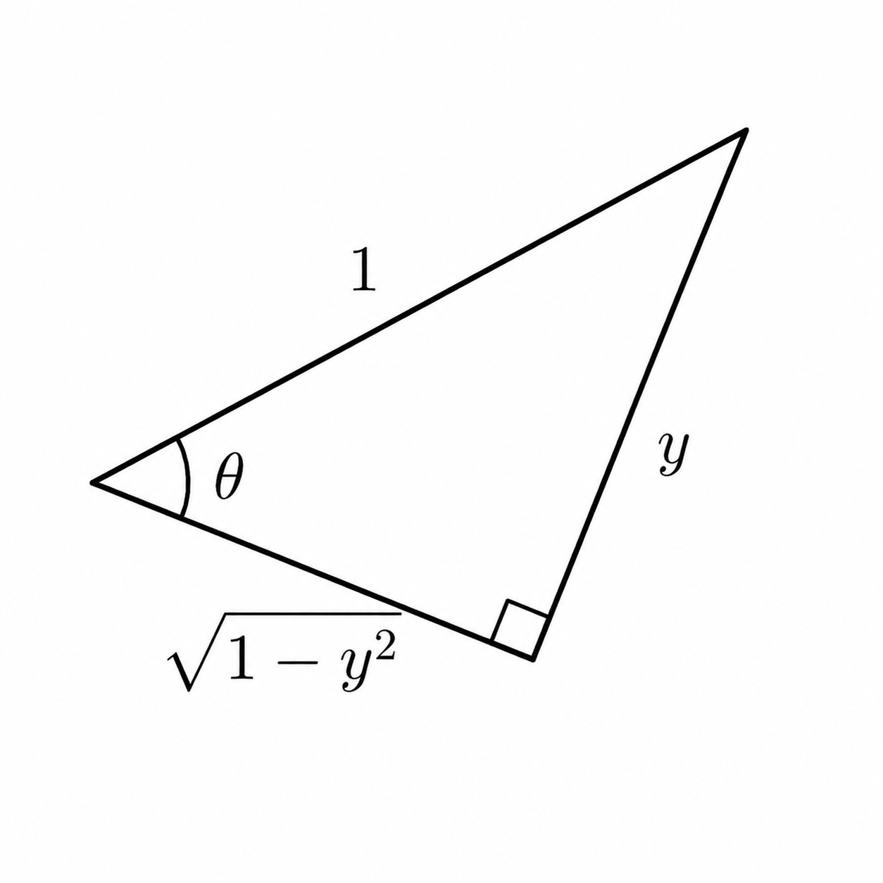
Therefore,
$$\frac{1}{2}\arcsin(y) + \frac{1}{2}y\sqrt{1 – y^2} = \frac{1}{2}x^2 + C.$$
Our final solution is then
$$\arcsin(y) + y\sqrt{1 – y^2} = x^2 + C.$$
The next example requires partial fraction decomposition, so you may wish to review the articles A Comprehensive Beginner’s Guide to Partial Fraction Decomposition and Partial Fraction Decomposition Integration Problems with Solutions: A Complete Tutorial for a refresher.
Example 5: Solve \( \frac{dy}{dx} = x(y – 1)(y + 2) \).
Solution: The equation is already in standard form. Separating variables, we have
$$\frac{1}{(y – 1)(y + 2)} dy = x dx.$$
Integrating both sides, we find
$$\int \frac{1}{(y – 1)(y + 2)} dy = \int x dx.$$
To evaluate the integral on the left-hand side, we use partial fraction decomposition. Setting up the partial fraction decomposition, we get
$$\frac{1}{(y – 1)(y + 2)} = \frac{A}{y – 1} + \frac{B}{y + 2}.$$
Next, multiplying both sides by \( (y – 1)(y + 2) \) gives
$$1 = A(y + 2) + B(y – 1).$$
Now we solve for the coefficients by choosing convenient values of y:
$$y = 1 \Rightarrow 1 = 3A \Rightarrow \frac{1}{3} = A$$
$$y = -2 \Rightarrow 1 = -3B \Rightarrow -\frac{1}{3} = B.$$
Thus
$$\frac{1}{(y – 1)(y + 2)} = \frac{1}{3}(\frac{1}{y – 1} – \frac{1}{y + 2}).$$
The integral is then
$$\frac{1}{3}\int \frac{1}{y – 1} – \frac{1}{y + 2} dy = \int x dx.$$
Therefore
$$\frac{1}{3}(\ln|y – 1| – \ln|y + 2|) = \frac{1}{2}x^2 + C.$$
Multiplying both sides by 3, we find
$$\ln|y – 1| – \ln|y + 2| = \frac{3}{2}x^2 + 3C.$$
This is equivalent to
$$\ln|y – 1| – \ln|y + 2| = \frac{3}{2}x^2 + C.$$
Simplifying the left-hand side, we get
$$\ln|\frac{y – 1}{y + 2}| = \frac{3}{2}x^2 + C.$$
In exponential form, this is
$$|\frac{y – 1}{y + 2}| = e^{\frac{3}{2}x^2 + C}.$$
Using exponential properties, we obtain
$$|\frac{y – 1}{y + 2}| = e^{\frac{3}{2}x^2}e^C.$$
This is equivalent to
$$|\frac{y – 1}{y + 2}| = Ce^{\frac{3}{2}x^2}.$$
Dropping the absolute value bars then gives
$$\frac{y – 1}{y + 2} = \pm Ce^{\frac{3}{2}x^2}.$$
This is equivalent to
$$\frac{y – 1}{y + 2} = Ce^{\frac{3}{2}x^2}.$$
Multiplying both sides by \( y + 2 \) we get
$$y – 1 = Ce^{\frac{3}{2}x^2}(y + 2).$$
Distributing gives
$$y – 1 = Ce^{\frac{3}{2}x^2}y + 2Ce^{\frac{3}{2}x^2}.$$
Adding \( 1 – Ce^{\frac{3}{2}x^2}y \) to both sides we find
$$y – Ce^{\frac{3}{2}x^2}y = 1 + 2Ce^{\frac{3}{2}x^2}.$$
Factoring out a y, this is
$$y(1 – Ce^{\frac{3}{2}x^2}) = 1 + 2Ce^{\frac{3}{2}x^2}.$$
Our final solution is then
$$y = \frac{1 + 2Ce^{\frac{3}{2}x^2}}{1 – Ce^{\frac{3}{2}x^2}}.$$
These examples illustrate how the separation of variables method combines naturally with many of the integration techniques encountered in calculus.
Conclusion
In this guide on separable differential equations explained step by step, we developed a complete framework for understanding and solving separable differential equations. We began by defining what separable differential equations are and learning how to recognize them. We then derived the separation of variables method from the general form of a separable differential equation, showing why moving the variables to opposite sides of the equation allows us to integrate and obtain a solution.
Next, we established a systematic procedure for solving separable differential equations. The process consists of identifying whether the equation is separable, separating the variables, integrating both sides, including the constant of integration, solving for y when possible, and applying any initial conditions.
The examples demonstrated that separable differential equations often require integration techniques beyond basic antiderivatives. Depending on the problem, you may need substitution, integration by parts, trigonometric substitution, or partial fraction decomposition after separating the variables. As a result, success with separable differential equations is closely connected to having a strong understanding of integration methods.
Further Reading
A Step-by-Step Tutorial on Linear Differential Equations with Examples and Solutions — Linear differential equations are another one of the basic differential equations you should be able to solve. This article covers these equations in depth.
