
Beginner’s Guide to Changing Variables in Double and Triple Integrals: Everything You Need to Know
In The Ultimate Step-by-Step Guide to Solving Integrals Using Substitution, we covered how to solve single-variable integrals using substitution. We extend this idea to multiple integrals in this beginner’s guide to changing variables in double and triple integrals. In multivariable calculus, changing variables is a powerful technique that can simplify both the integrand and the region of integration.
This guide will teach you exactly when and how to change variables in double and triple integrals. We’ll cover the underlying theory, walk through the role of the Jacobian determinant, and demonstrate the process through examples. By the end, you’ll be able to tackle a wide range of problems.
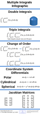
This article is part of a five-part series on evaluating multiple integrals. The following infographic illustrates this topic.
Why Change Variables in Multiple Integrals?
Changing variables in double and triple integrals involves rewriting an integral in terms of new variables that better suit the structure of the region or the function being integrated. Here are the reasons why changing variables can be helpful:
- Simplifying the Region of Integration – Some regions are defined by boundaries that are difficult to describe using the original variables. For instance, if an area is bounded by expressions like \( x + y = \text{constant} \) or \( x – y = \text{constant} \), switching to new variables such as \( u = x + y \) and \( v = x – y \) can transform an angled region into a rectangle, making it much simpler to evaluate the integral.
- Simplifying the Integrand – The integrand may have a complicated form that becomes simpler after changing variables. For example, expressions like \( (x – y)^2 \) or \( x^2 – y^2 \) might factor or reduce nicely when written in terms of \( u = x – y \) and \( v = x + y \). The right substitution can often transform a difficult integrand into a much simpler one.
The Jacobian Determinant
The Jacobian tells us how much a small area or volume element is stretched or compressed when we move from the original variables \( (x, y) \) or \( (x, y, z) \) to new variables \( (u, v) \) or \( (u, v, w) \). It acts as a scaling factor that corrects for this distortion, ensuring that the value of the integral remains the same in the new variables. The Jacobian Matrix consists of partial derivatives. If you need a review of partial derivatives, please refer to The Ultimate Beginner’s Guide to Partial Derivatives with Step-by-Step Examples.
The Jacobian Matrix
Let’s say you are changing variables in a double integral using the transformation:
$$x = x(u, v), \quad y = y(u, v),$$
The Jacobian matrix is
$$J = \begin{bmatrix}
\frac{\partial x}{\partial u} & \frac{\partial x}{\partial v} \\
\frac{\partial y}{\partial u} & \frac{\partial y}{\partial v}
\end{bmatrix},$$
and the Jacobian determinant is
$$\frac{\partial(x, y)}{\partial(u, v)} =
\begin{vmatrix}
\frac{\partial x}{\partial u} & \frac{\partial x}{\partial v} \\
\frac{\partial y}{\partial u} & \frac{\partial y}{\partial v}
\end{vmatrix}.$$
This determinant tells you how much a tiny area in the \( uv \)-plane is stretched when mapped into the \( xy \)-plane.
If you’re unfamiliar with computing determinants, especially of \( 2 \times 2 \) or \( 3 \times 3 \) matrices, check out my article How to Find the Determinant of a Matrix Step by Step: A Complete Beginner’s Guide.
In triple integrals, the Jacobian is the \( 3 \times 3 \) matrix
$$J = \begin{bmatrix}
\frac{\partial x}{\partial u} & \frac{\partial x}{\partial v} & \frac{\partial x}{\partial w} \\
\frac{\partial y}{\partial u} & \frac{\partial y}{\partial v} & \frac{\partial y}{\partial w} \\
\frac{\partial z}{\partial u} & \frac{\partial z}{\partial v} & \frac{\partial z}{\partial w}
\end{bmatrix},$$
and the Jacobian determinant is
$$\frac{\partial(x, y, z)}{\partial(u, v, w)} = \begin{vmatrix}
\frac{\partial x}{\partial u} & \frac{\partial x}{\partial v} & \frac{\partial x}{\partial w} \\
\frac{\partial y}{\partial u} & \frac{\partial y}{\partial v} & \frac{\partial y}{\partial w} \\
\frac{\partial z}{\partial u} & \frac{\partial z}{\partial v} & \frac{\partial z}{\partial w}
\end{vmatrix}.$$
This gives you the scale factor for volume elements under the transformation.
Putting It All Together
When you change variables in an integral, it becomes
$$\iint_R f(x, y) \, dxdy = \iint_{R’} f(x(u, v), y(u, v)) \left| \frac{\partial(x, y)}{\partial(u, v)} \right| \, dudv,$$
or
$$\iiint_R f(x, y, z) \, dxdydz = \iiint_{R’} f(x(u, v, w), y(u, v, w), z(u, v, w)) \left| \frac{\partial(x, y, z)}{\partial(u, v, w)} \right| \, dudvdw.$$
In the next section, we’ll give guidelines for choosing a substitution.
How to Choose the Right Substitution
Choosing the correct substitution is the most challenging step when changing variables in double and triple integrals. A well-chosen change of variables can turn a complicated region into a rectangle or box, simplify the integrand, or both. Here are some guidelines for selecting new variables:
Look at the Boundary Curves or Surfaces
Start by examining the equations that define the boundaries of the region of integration. If those boundaries involve expressions like \( x + y \), \( x – y \), or \( xy \), try using those as your new variables.
Identify Patterns in the Integrand
Next, analyze the integrand. If the integrand contains terms like \( (x – y)^2 \), \( x^2 – y^2 \), or \( x + y \), those patterns can often be simplified by making substitutions that reflect those expressions.
In the next section, we’ll review the step-by-step procedure for changing variables.
Step-by-Step Process for Changing Variables
Now that you understand why changing variables can help and how to choose a substitution, let’s walk through the process. The general steps remain the same whether you’re working with a double or triple integral. This section outlines each step. The process is similar to what we did in the article, Step-by-Step Tutorial on How to Use Polar, Cylindrical, and Spherical Coordinates in Integrals, but more general.
Step 1: Choose an Appropriate Substitution
Look at the region and the integrand to decide on new variables \( u, v \) or \( u, v, w \). Your goal is to simplify the region of integration, the integrand, or both. Use the strategies from the previous section to guide your choice.
Step 2: Express the Original Variables in Terms of the New Ones
Once you’ve chosen your substitution, rewrite \( x, y \) or \( x, y, z \) as functions of the new variables.
Step 3: Compute the Jacobian Determinant
Calculate the Jacobian determinant. This determinant represents the local scaling factor between the old and new variables. Don’t forget to take the absolute value of the Jacobian determinant in your final integral.
Step 4: Rewrite the Region in Terms of the New Variables
Convert the original bounds of integration into bounds in the \( uv \) or \( uvw \) coordinate system. This may require sketching the transformed region as we did in The Ultimate Step-by-Step Guide to Changing Order of Integration with Examples.
Step 5: Rewrite the Integrand
Substitute the expressions for \( x, y \), or \( x, y, z \) into the integrand. Then multiply the entire integrand by the absolute value of the Jacobian determinant. This gives you the new integrand in the \( uv \) or \( uvw \) variables.
Step 6: Set Up and Evaluate the New Integral
Write out the new iterated integral with the updated integrand and new limits of integration. Then evaluate using the techniques covered in A Step-by-Step Beginner’s Tutorial for Double and Triple Integrals in Calculus and Double and Triple Integrals Explained with Examples for General Regions: A Complete Beginner’s Guide.
By following these steps, you can change variables. In the following sections, we’ll apply this whole process to worked examples of double and triple integrals using substitutions.
Worked Out Examples
Let’s now apply change of variables to two examples that will demonstrate how to choose a substitution, compute the Jacobian, rewrite the region and integrand, and evaluate the new integral. These integrals will use techniques covered in the articles Basic Integration Problems for Beginners and How to Integrate Products of Trigonometric Functions: Techniques and Tricks.
Example 1: Evaluate:
(a) \( \iint_R (x – y)^2 \, dxdy \) where \( R \) is the parallelogram with vertices \( (0, 0), (2, 2), (3, 1), (1, -1) \).
(b) \( \iiint_E (x^2 + y^2 + z^2) \, dV \), where \( E \) is the ellipsoid defined by \( \frac{x^2}{4} + \frac{y^2}{9} + \frac{z^2}{16} \leq 1 \).
Solution: (a) \( \iint_R (x – y)^2 \, dxdy \) where \( R \) is the parallelogram with vertices \( (0, 0), (2, 2), (3, 1), (1, -1) \).
Below is a sketch of the region.
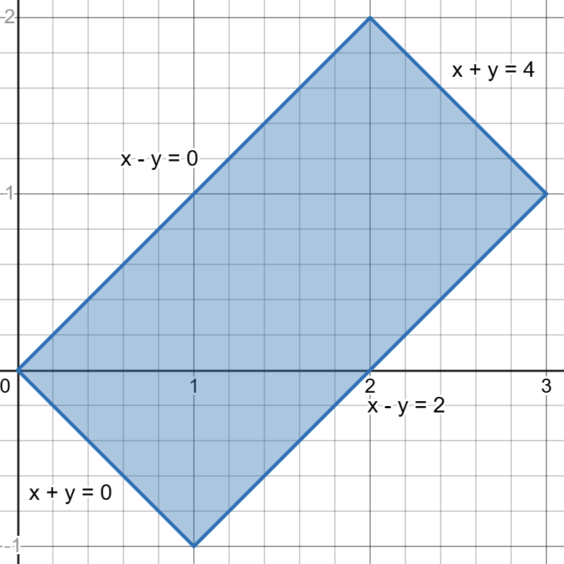
This region is bounded by the lines x – y = 0, x + y = 0, x – y = 2, and x + y = 4. We will use the change of variables
$$u = x – y, \quad v = x + y.$$
Solving for x and y gives
$$x = \frac{u + v}{2}, \quad y = \frac{v – u}{2}.$$
The Jacobian for this transformation is
$$J = \begin{bmatrix}
\frac{\partial}{\partial u}\frac{u + v}{2} & \frac{\partial}{\partial v}\frac{u + v}{2} \\
\frac{\partial}{\partial u}\frac{v – u}{2} & \frac{\partial}{\partial v}\frac{v – u}{2}
\end{bmatrix}.$$
Computing the partial derivatives, we get
$$J = \begin{bmatrix}
\frac{1}{2} & \frac{1}{2} \\
-\frac{1}{2} & \frac{1}{2}
\end{bmatrix}.$$
To find the determinant, we apply the determinant formula for 2×2 matrices, which gives
$$\begin{vmatrix}
\frac{1}{2} & \frac{1}{2} \\
-\frac{1}{2} & \frac{1}{2}
\end{vmatrix}
= \frac{1}{2}\frac{1}{2} – \frac{1}{2}(-\frac{1}{2}).$$
Simplifying we get
$$\begin{vmatrix}
\frac{1}{2} & \frac{1}{2} \\
-\frac{1}{2} & \frac{1}{2}
\end{vmatrix}
= \frac{1}{4} + \frac{1}{4}.$$
Adding, we obtain
$$\begin{vmatrix}
\frac{1}{2} & \frac{1}{2} \\
-\frac{1}{2} & \frac{1}{2}
\end{vmatrix}
= \frac{1}{2}.$$
We now compute the limits. The transformed region is shown below.
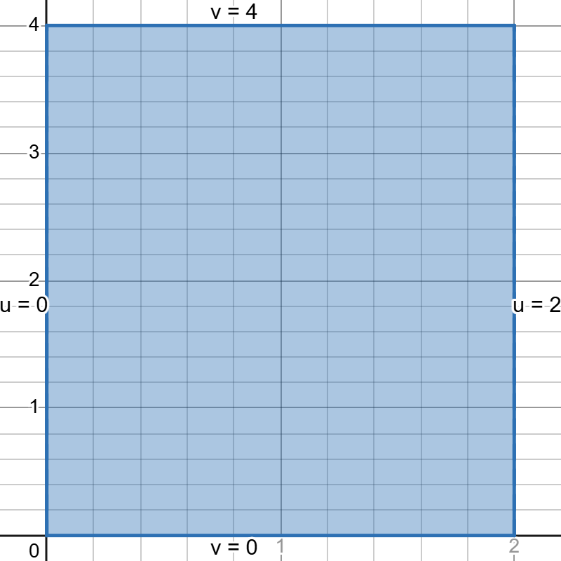
We can describe this region as
$$\{ (u,v) | 0 \leq u \leq 2, 0 \leq v \leq 4 \}.$$
Hence, our new integral is
$$\frac{1}{2} \int_0^4 \int_0^2 u^2dudv.$$
The inner integral is with respect to u, so we treat \( v \) as a constant and integrate with respect to \( u \) to get
$$\frac{1}{6} \int_0^4 u^3 |_0^2 dv.$$
Applying the Fundamental Theorem of Calculus gives
$$\frac{4}{3} \int_0^4 dv.$$
Now, we integrate with respect to v to obtain
$$\frac{4}{3} v|_0^4.$$
Applying the Fundamental Theorem of Calculus again, we arrive at a final answer of
$$\frac{16}{3}.$$
(b) \( \iiint_E (x^2 + y^2 + z^2) \, dV \), where \( E \) is the ellipsoid defined by \( \frac{x^2}{4} + \frac{y^2}{9} + \frac{z^2}{16} \leq 1 \).
Below is a sketch of the region.
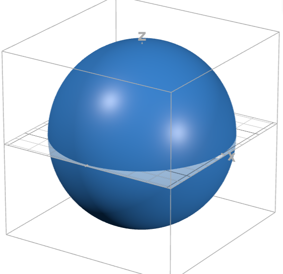
This region is the ellipsoid with axes of symmetry of lengths 2, 3, and 4. We will use the change of variables
$$x = 2u, \quad y = 3v, \quad z = 4w.$$
The Jacobian for this transformation is
$$J = \begin{bmatrix}
\frac{\partial}{\partial u}2u & \frac{\partial}{\partial v}2u & \frac{\partial}{\partial w}2u \\
\frac{\partial}{\partial u}3v & \frac{\partial}{\partial v}3v & \frac{\partial}{\partial w}3v \\
\frac{\partial}{\partial u}4w & \frac{\partial}{\partial v}4w & \frac{\partial}{\partial w}4w
\end{bmatrix}.$$
Computing the partial derivatives, we get
$$J = \begin{bmatrix}
2 & 0 & 0 \\
0 & 3 & 0 \\
0 & 0 & 4
\end{bmatrix}.$$
To find the determinant, we apply the determinant formula for triangular matrices, which gives
$$\begin{vmatrix}
2 & 0 & 0 \\
0 & 3 & 0 \\
0 & 0 & 4
\end{vmatrix} = (2)(3)(4).$$
Multiplying, we obtain
$$\begin{vmatrix}
2 & 0 & 0 \\
0 & 3 & 0 \\
0 & 0 & 4
\end{vmatrix} = 24.$$
We now compute the limits. The transformed region is shown below
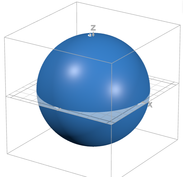
This is the unit sphere centered at the origin. Hence, our new integral is
\( 24\iiint_E (4u^2 + 9v^2 + 16w^2) \, dV \), where \( E \) is the sphere defined by \( u^2 + v^2 + w^2 \leq 1 \).
We can describe the region in spherical coordinates as
$$ \{ (\rho,\theta,\phi) | 0 \leq \rho \leq 1, 0 \leq \theta \leq 2\pi, 0 \leq \phi \leq \pi \}.$$
Plugging in the substitutions \( u = \rho\sin\phi\cos\theta \), \( v = \rho\sin\phi\sin\theta \), \( w = \rho\cos\phi \), and \( dudvdw = \rho^2\sin\phi d\rho d\theta d\phi \), our new integral is
$$24\int_0^{\pi} \int_0^{2\pi} \int_0^1 (4\rho^2\sin^2\phi\cos^2\theta + 9\rho^2\sin^2\phi\sin^2\theta + 16\rho^2\cos^2\phi) \rho^2\sin\phi d\rho d\theta d\phi.$$
Distributing, \( \rho^2\sin\phi \) gives
$$24\int_0^{\pi} \int_0^{2\pi} \int_0^1 4\rho^4\sin^3\phi\cos^2\theta + 9\rho^4\sin^3\phi\sin^2\theta + 16\rho^4\sin\phi\cos^2\phi d\rho d\theta d\phi.$$
Factoring out \( \rho^4 \) we obtain
$$24\int_0^{\pi} \int_0^{2\pi} \int_0^1 \rho^4(4\sin^3\phi\cos^2\theta + 9\sin^3\phi\sin^2\theta + 16\sin\phi\cos^2\phi) d\rho d\theta d\phi.$$
The inner integral is with respect to \( \rho \), so we treat \( \theta \) and \( \phi \) as constants and integrate with respect to \( \rho \) to get
$$\frac{24}{5}\int_0^{\pi} \int_0^{2\pi} \rho^5|_0^1(4\sin^3\phi\cos^2\theta + 9\sin^3\phi\sin^2\theta + 16\sin\phi\cos^2\phi) d\theta d\phi.$$
Applying the Fundamental Theorem of Calculus gives
$$\frac{24}{5}\int_0^{\pi} \int_0^{2\pi} 4\sin^3\phi\cos^2\theta + 9\sin^3\phi\sin^2\theta + 16\sin\phi\cos^2\phi d\theta d\phi.$$
We now integrate with respect to \( \theta \) while treating \( \phi \) as a constant. To accomplish this, we apply the power-reducing identity for sine and cosine. This gives
$$\frac{12}{5}\int_0^{\pi} \int_0^{2\pi} 4\sin^3\phi(1 + \cos2\theta) + 9\sin^3\phi(1 – \cos2\theta) + 16\sin\phi\cos^2\phi d\theta d\phi.$$
Integrating gives
$$\frac{12}{5}\int_0^{\pi} 4\sin^3\phi(\theta + \frac{1}{2}\sin2\theta) + 9\sin^3\phi(\theta – \frac{1}{2}\sin2\theta) + 16\theta\sin\phi\cos^2\phi|_0^{2\pi} d\phi.$$
Applying the Fundamental Theorem of Calculus again, we arrive at
$$\frac{24\pi}{5}\int_0^{\pi} 13\sin^3\phi + 16\sin\phi\cos^2\phi d\phi.$$
To evaluate the remaining integral, we begin by factoring out a sine to obtain
$$\frac{24\pi}{5}\int_0^{\pi} \sin\phi(13\sin^2\phi + 16\cos^2\phi d\phi.$$
Applying the Pythagorean identity, we get
$$\frac{24\pi}{5}\int_0^{\pi} \sin\phi(13(1 – \cos^2\phi) + 16\cos^2\phi) d\phi.$$
This simplifies to
$$\frac{24\pi}{5}\int_0^{\pi} \sin\phi(13 + 3\cos^2\phi) d\phi.$$
Let \( u = \cos\phi \) then \( du = -\sin\phi d\phi \) which implies \( -du = \sin\phi d\phi \). The new limits are \( \cos{0} = 1 \) and \( \cos\pi = -1 \). Hence, we have
$$-\frac{24\pi}{5}\int_1^{-1} 13 + 3u^2 du.$$
Now, we integrate with respect to u to obtain
$$-\frac{24\pi}{5}(13u + u^3)|_1^{-1}.$$
Applying the Fundamental Theorem of Calculus once again, we arrive at a final answer of
$$\frac{672\pi}{5}.$$
In both examples, a substitution transformed a difficult region into a simpler one.
Conclusion
Changing variables in double and triple integrals is a powerful tool for simplifying complicated integrands and regions by mapping them into simpler forms. In this beginner’s guide to changing variables in double and triple integrals, we explored the process behind change of variable, and how to compute the Jacobian, and you saw fully worked examples that show how these techniques work in practice.
Further Reading
Step-by-Step Tutorial on How to Use Polar, Cylindrical, and Spherical Coordinates in Integrals – Changing variables is a generalization of changing coordinates. For a deeper understanding, I recommend reading this article again.
