How to Calculate Limits in Calculus: Everything You Need to Know
If you’re starting with calculus, you’re probably learning to calculate limits. Limits are the foundation of calculus and are used to define the concepts of continuity, derivatives, and integrals. Limits are a valuable tool, whether you’re looking at the behavior of a function near a particular point or exploring what happens as x tends to infinity. This guide will walk you through everything you need to know about calculating limits. You’ll learn the difference between finite and infinite limits and how to calculate limits both at specific points and as x approaches infinity. We’ll cover algebraic techniques, the squeeze theorem, L’Hôspital’s Rule, and even how to use Taylor series to compute limits.
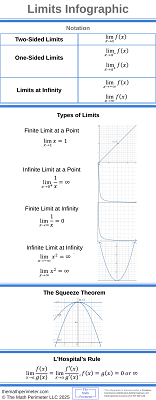
The following infographic illustrates the concepts covered in this article.
What Is a Limit?
A limit describes the behavior of a function as the input \( x \) gets close to a specific value, even if the function is undefined at that value. In other words, it answers the question, What value does the function approach as \( x \) gets closer and closer to a specific point?
Limit Notation
There are several forms of limit notation you’ll encounter:
Two-sided limit: \( \lim_{x \to a} f(x) \).
This represents the value \( f(x) \) approaches as \( x \) gets close to \( a \) from both sides.
One-sided limits: \( \lim_{x \to a^-} f(x) \) and \( \lim_{x \to a^+} f(x) \).
This represents the value \( f(x) \) approaches as \( x \) gets close to \( a \) from the left and right sides respectively.
Limits at infinity: \( \lim_{x \to \infty} f(x) \) and \( \lim_{x \to -\infty} f(x) \).
These describe the behavior of a function as the magnitude of \( x \) becomes very large in the positive or negative direction.
Understanding how to read and interpret these notations is the first step toward mastering limits. In the next section, we’ll look at the different limits you’ll encounter.
Types of Limits
Not all limits behave the same way. Sometimes, the function approaches a finite number; and sometimes, it heads toward infinity. Limits can be taken at a specific point or as the input becomes infinitely large. Here are the main types of limits you’ll encounter.
Finite Limits at Finite Points
A finite limit at a finite point occurs when the input \( x \) approaches a specific point, and the function approaches a finite value.
Example 1: Calculate \( \lim_{x \to 3} (2x + 1) \).
Solution: As \( x \) gets closer to 3, the value of the function gets closer to
$$\lim_{x \to 3} (2x + 1) = 2(3) + 1.$$
Multiplying gives
$$\lim_{x \to 3} (2x + 1) = 6 + 1.$$
Adding we arrive at a final answer of
$$\lim_{x \to 3} (2x + 1) = 7.$$
This is the most straightforward type of limit. If the function is continuous at that point, you can evaluate the limit by plugging in the value of \( x \).
Infinite Limits at Finite Points
An infinite limit at a finite point happens when the function increases or decreases without bound as \( x \) approaches a specific value. This generally implies the existence of a vertical asymptote.
Example 2: Calculate \( \lim_{x \to 0^+} \frac{1}{x} \).
Solution: As \( x \) approaches 0 from the right, the values of \( \frac{1}{x} \) grows larger and remains positive, so we have a final answer of
$$\lim_{x \to 0^+} \frac{1}{x} = \infty.$$
Finite Limits at Infinity
A finite limit at infinity describes what happens to a function as the magnitude of \( x \) becomes very large.
Example 3: Calculate \( \lim_{x \to \infty} \frac{1}{x} \).
Solution: As \( x \) increases, \( \frac{1}{x} \) gets smaller, hence we have a final answer of
$$\lim_{x \to \infty} \frac{1}{x} = 0.$$
This type of limit helps you find horizontal asymptotes and analyze end behavior.
Infinite Limits at Infinity
Sometimes, a function grows without bound as the magnitude of \( x \) becomes very large. These are infinite limits at infinity.
Example 4: Calculate \( \lim_{x \to \infty} x^2 \).
Solution: As \( x \) increases, so does \( x^2 \), and it does not approach an upper bound, so we have a final answer of
$$\lim_{x \to \infty} x^2 = \infty.$$
Understanding these four types of limits will help you identify what kind of strategy to use when calculating limits. In the next section, we’ll learn how to find limits using algebraic techniques.
How to Calculate Limits Algebraically
When calculating a limit, we generally compute it using algebraic methods first. These include direct substitution, factoring, and rationalizing. Let’s go through each technique with examples so you can see how they work.
Direct Substitution
If the function is continuous at the point, you can plug in the value of \( x \). We did this in the previous section.
Factoring
When direct substitution gives an indeterminate form like \( \frac{0}{0} \), try factoring.
Example 5: Calculate \( \lim_{x \to 3} \frac{x^2 – 9}{x – 3} \).
Solution: Attempting direct substitution gives the indeterminate form \( \frac{0}{0} \). We proceed by factoring the numerator to get
$$\lim_{x \to 3} \frac{(x – 3)(x + 3)}{x – 3}.$$
Simplifying gives
$$\lim_{x \to 3} x + 3.$$
Substituting in \( x = 3 \) we obtain
$$3 + 3.$$
Adding we arrive at a final answer of
$$6.$$
Rationalizing
This technique is useful when dealing with square roots.
Example 6: Calculate \( \lim_{x \to 4} \frac{\sqrt{x} – 2}{x – 4} \).
Solution: Attempting direct substitution gives the indeterminate form \( \frac{0}{0} \). We proceed by rationalizing the numerator to get
$$\lim_{x \to 4} \frac{(\sqrt{x} – 2)(\sqrt{x} + 2)}{(x – 4)(\sqrt{x} + 2)}.$$
This is equivalent to
$$\lim_{x \to 4} \frac{x – 4}{(x – 4)(\sqrt{x} + 2)}.$$
Simplifying gives
$$\lim_{x \to 4} \frac{1}{\sqrt{x} + 2}.$$
Substituting in \( x = 4 \) we obtain
$$\frac{1}{\sqrt{4} + 2}.$$
Taking the square root, we get
$$\frac{1}{2 + 2}.$$
Adding we arrive at a final answer of
$$\frac{1}{4}.$$
Limits at infinity
Example 7: Calculate:
(a) \( \lim_{x \to \infty} x^2 – 6x \)
(b) \( \lim_{x \to \infty} \frac{x^2 + 6x + 10}{x^2 + 7x + 12} \)
Solution: (a) \( \lim_{x \to \infty} x^2 – 6x \)
Attempting direct substitution gives the indeterminate form \( \infty – \infty \). We proceed by factoring out an \( x^2 \) to get
$$\lim_{x \to \infty} x^2(1 – \frac{6}{x}).$$
As \( x \) approaches infinity, \( 1 – \frac{6}{x} \) approaches 1, while \( x^2 \) grows without bound so our final answer is
$$\lim_{x \to \infty} (x^2 – 6x) = \infty.$$
(b) \( \lim_{x \to \infty} \frac{x^2 + 6x + 10}{x^2 + 7x + 12} \)
Attempting direct substitution gives the indeterminate form \( \frac{\infty}{\infty} \). We proceed by factoring an \( x^2 \) out of the numerator and denominator to get
$$\lim_{x \to \infty} \frac{x^2(1 + \frac{6}{x} + \frac{10}{x^2})}{x^2(1 + \frac{7}{x} + \frac{12}{x^2})}.$$
Simplifying we obtain
$$\lim_{x \to \infty} \frac{1 + \frac{6}{x} + \frac{10}{x^2}}{1 + \frac{7}{x} + \frac{12}{x^2}}.$$
As x approaches infinity, both the numerator and denominator approach 1, so
$$\lim_{x \to \infty} \frac{x^2 + 6x + 10}{x^2 + 7x + 12} = 1.$$
Algebraic techniques are the first tools you should try when solving limit problems. When these don’t work, you’ll need to use more advanced methods, such as L’Hôspital’s Rule, the Squeeze Theorem, or Taylor Series, which are covered in the next few sections.
How to Use the Squeeze Theorem to Calculate Limits
The Squeeze Theorem can be used to evaluate limits when other techniques won’t work.
Statement of the Squeeze Theorem
If three functions satisfy the inequality
$$f(x) \leq g(x) \leq h(x)$$
for all \( x \) near \( a \), and
$$\lim_{x \to a} f(x) = \lim_{x \to a} h(x) = L,$$
then
$$\lim_{x \to a} g(x) = L.$$
In other words, if a function is “squeezed” between two others that share the same limit, it must also approach that same limit.
Squeeze Theorem Example
Example 8: Calculate \( \lim_{x \to 0} x^2 \sin\left(\frac{1}{x}\right) \).
Solution: We know that
$$-1 \leq \sin\left(\frac{1}{x}\right) \leq 1.$$
Multiplying through by \( x^2 \) we obtain
$$-x^2 \leq x^2 \sin\left(\frac{1}{x}\right) \leq x^2.$$
Since \( \lim_{x \to 0} (-x^2) = 0 \) and \( \lim_{x \to 0} x^2 = 0 \) we conclude that
$$\lim_{x \to 0} x^2 \sin\left(\frac{1}{x}\right) = 0.$$
The Squeeze Theorem is especially helpful when dealing with oscillating or bounded functions multiplied by something that goes to zero. The squeeze theorem is a valuable tool if you can squeeze a difficult expression between two simpler expressions with the same limit.
How to Use L’Hôspital’s Rule to Calculate Limits
When you encounter an indeterminate form like \( \frac{0}{0} \) or \( \frac{\infty}{\infty} \), L’Hôspital’s Rule is one of the most powerful tools you can use to evaluate the limit. It’s based on differentiation, so make sure you’re comfortable taking derivatives, and if you need a refresher, please check out my article How to Differentiate a Function Step by Step: A Beginner’s Guide.
Statement of L’Hôspital’s Rule
If \( \lim_{x \to a} \frac{f(x)}{g(x)} = \frac{0}{0} \) or \( \lim_{x \to a} \frac{f(x)}{g(x)} = \frac{\infty}{\infty} \), and both \( f(x) \) and \( g(x) \) are differentiable near \( a \), then
$$\lim_{x \to a} \frac{f(x)}{g(x)} = \lim_{x \to a} \frac{f'(x)}{g'(x)},$$
provided the limit on the right-hand side exists.
L’Hôspital’s Rule Examples
Example 9: Calculate:
(a) \( \lim_{x \to \infty} \frac{\ln x}{x} \)
(b) \( \lim_{x \to 0^+} x^x \).
Solution: (a) \( \lim_{x \to \infty} \frac{\ln x}{x} \).
Attempting direct substitution gives the indeterminate form \( \frac{\infty}{\infty} \). We proceed using L’Hôspital’s Rule to get
$$\lim_{x \to \infty} \frac{\ln x}{x} = \lim_{x \to \infty} \frac{1/x}{1}.$$
Simplifying gives
$$\lim_{x \to \infty} \frac{\ln x}{x} = \lim_{x \to \infty} \frac{1}{x}.$$
Taking the limit, we arrive at a final answer of
$$\lim_{x \to \infty} \frac{\ln x}{x} = 0.$$
(b) \( \lim_{x \to 0^+} x^x \)
Attempting direct substitution gives the indeterminate form \( 0^0 \). We proceed using properties of exponents and logarithms to get
$$\lim_{x \to 0^+} e^{\ln{x^x}}.$$
This is equivalent to
$$\lim_{x \to 0^+} e^{x\ln{x}}.$$
Using properties of limits gives
$$e^{\lim_{x \to 0^+} x\ln{x}}.$$
Another application of direct substitution gives the indeterminate form \( 0\infty \). We proceed by rewriting x using negative exponents to obtain
$$e^{\lim_{x \to 0^+}} \frac{\ln{x}}{x^{-1}}.$$
Trying direct substitution a third time gives the indeterminate form \( \frac{\infty}{\infty} \). We can now use L’Hôspital’s Rule to arrive at
$$e^{\lim_{x \to 0^+}} \frac{\frac{1}{x}}{-x^{-2}}.$$
Simplifying gives
$$e^{-\lim_{x \to 0^+} x}.$$
Taking the limit, we get
$$e^0.$$
Evaluating the exponential, we obtain a final answer of
$$1.$$
L’Hôspital’s Rule is one of the most used tools for evaluating limits of indeterminate form. When used alongside techniques like algebraic manipulation, it becomes even more valuable.
How to Use Taylor Series to Compute Limits
In some cases, limits involve functions that make them difficult to evaluate using algebraic methods or L’Hôspital’s Rule. That’s where Taylor series can help.
Taylor series allow us to express functions as an infinite power series, which can make it easier to analyze behavior near a specific point.
What Is a Taylor Series?
The Taylor series of a function \( f(x) \) centered at \( a \) is
$$f(x) = \sum_{n=0}^\infty \frac{f^{(n)}(a)}{n!} (x – a)^n.$$
When \( a = 0 \), this is called a Maclaurin series:
$$f(x) = \sum_{n=0}^\infty \frac{f^{(n)}(0)}{n!} x^n.$$
Some common Maclaurin series include:
$$e^x = \sum_{n=0}^{\infty} \frac{x^n}{n!}$$
$$\sin x = \sum_{n=0}^{\infty} (-1)^n \frac{x^{2n+1}}{(2n+1)!}$$
$$\cos x = \sum_{n=0}^{\infty} (-1)^n \frac{x^{2n}}{(2n)!}.$$
Taylor Series Example
Example 10: Evaluate \( \lim_{x \to 0} \frac{1 – \cos x}{x^2} \).
Solution: Substitute the Maclaurin series for \( \cos x \) into the expression to obtain
$$\lim_{x \to 0} \frac{1 – \sum_{n=0}^{\infty} (-1)^n \frac{x^{2n}}{(2n)!}}{x^2}.$$
This is equivalent to
$$\lim_{x \to 0} \frac{1 – (1 + \sum_{n=1}^{\infty} (-1)^n \frac{x^{2n}}{(2n)!})}{x^2}.$$
Simplifying gives
$$\lim_{x \to 0} \frac{-\sum_{n=1}^{\infty} (-1)^n \frac{x^{2n}}{(2n)!}}{x^2}.$$
Dividing by \( x^2 \) we get
$$-\lim_{x \to 0} \sum_{n=1}^{\infty} (-1)^n \frac{x^{2n – 2}}{(2n)!}.$$
This is equivalent to
$$-\lim_{x \to 0} (-\frac{1}{2} + \sum_{n=2}^{\infty} (-1)^n \frac{x^{2n – 2}}{(2n)!}).$$
Taking the limit, we arrive at a final answer of
$$\frac{1}{2}.$$
Taylor series are useful tools in all of mathematics. This is not the last time we’ll see them.
Conclusion
Calculating limits is one of the most important skills in calculus. In this guide, you learned how to calculate limits. Whether you’re dealing with finite or infinite limits, limits at a point or at infinity, mastering various techniques will give you the tools you need to compute any limit.
Further Reading
How to Differentiate a Function Step by Step: A Beginner’s Guide – Now that you can calculate limits, you are ready to learn about derivatives.
